⚠️ Important Notice About Translation
This content is translated using Google Translate and can be accessed in approximately 30+ languages worldwide, in order to make the content more accessible to non-English speakers.
However, due to the limitations of machine translation, many sentences may contain unnatural phrasing, incorrect terminology, or misinterpretation of the original meaning—especially in technical or philosophical contexts.
Please be aware that this translation is not professionally edited and may not fully reflect the precise intent or nuance of the original document.
For the most accurate understanding, we strongly recommend referring to the original English version of this paper, which represents the author's intended wording and conceptual clarity.
📌 Publication Status Note — September 2026
This manuscript is made available here as a project-site working manuscript.
Following OpenAI’s September 8, 2026 announcement of a proposed resolution of the Navier–Stokes Millennium Prize Problem, we have chosen to temporarily defer submission of this work to public preprint repositories and other archival channels while the mathematical community evaluates the result and while we reconsider its relationship to CJM–Navier.
CJM–Navier asks a different question: whether the structural fate of a flow—regular continuation or breakdown—can be discriminated without sequentially generating its future trajectory.
The manuscript is preserved here in its present form to document the state of the research at this time.
Please note that, as this is not the final published version, it may contain typographical or other errors.
On Structural Stability:
Atemporal Persistence of Navier–Stokes Flow
in Nonlinear Continua
Keunsoo Yoon  Independent Research Group (Seoul, Republic of Korea)
austiny@gatech.edu, austiny@snu.ac.kr
Independent Research Group (Seoul, Republic of Korea)
austiny@gatech.edu, austiny@snu.ac.kr
Sep 26, 2026
Abstract
The three-dimensional Navier–Stokes existence and smoothness problem is usually posed as a
question of temporal continuation: can a smooth flow remain regular for all time, or can finite-time
singularity occur? This paper asks a complementary question: must global regular continuation
be established through sequential trajectory generation, or can its admissibility be structurally
discriminated without knowing the future trajectory?
We examine this question within the atemporal complexity class O(J) and the Changbal
Jump Machine (CJM) framework. Physical evolution remains temporal, but CJM–Navier separates
temporal generation from structural discrimination. Independently generated flow snapshots
are converted into finite structural representations using vortex-stretching and viscous-control
information and evaluated through a fixed CJM core. The present construction is an operational
precursor to the stronger TRUE/FALSE discrimination of global regular continuation.
A finite three-dimensional Taylor–Green probe shows a marked reduction in instantaneous
structural control as Reynolds number increases, while the fixed-core CJM output retains persistent
but reorganized spatial structure. Small divergence-free symmetry-breaking perturbations preserve
the principal organization while revealing regions of enhanced structural susceptibility, where
comparatively smooth physical perturbations produce larger changes in the CJM response.
These results do not resolve global smoothness or finite-time singularity. They provide
preliminary evidence that regular continuation can be studied not only as temporal survival of a
trajectory, but also through the structural organization of what remains admissible before that
trajectory is known.
Keywords: Atemporal Discrimination; Changbal Jump Machine (CJM); O(J); Navier–Stokes Equations;
Structural Persistence; Structural Admissibility; Taylor–Green Vortex; 3SAT; 창발
The Master Manifesto. We propose a shift in addressing the Millennium Prize Problems
from exclusively formal, time-bound proof toward structural and physically discriminable
experimentation, reinterpreting mathematical conjectures not as statements requiring
asymptotic derivation but as questions of realizability within a structured, non-temporal state
space.
This series originates from the P versus NP problem, reformulated through the Changbal
Atemporal Equation, P a NP\(^{J}\), and evaluated by the Changbal Jump Machine (CJM). The term
Changbal is derived from the Korean conceptual notion of = and denotes a discontinuous
structural transition beyond constraint boundaries, distinct from gradual emergence; within
this framework, solvability is defined by structural admissibility rather than computational
effort.
The technical foundations of the O(J) state space, the Changbal Atemporal Equation, and the
CJM architecture have been developed and analyzed in detail in prior work [1]; accordingly,
these elements are treated here as established primitives, and the present paper focuses
exclusively on their application to a specific conjecture rather than on re-deriving or extending
the underlying formalism.
1 Introduction
The three-dimensional Navier–Stokes equations describe one of the most fundamental nonlinear systems in
mathematical physics [2],
\begin{equation} \frac {\partial u}{\partial t} +(u\cdot \nabla )u = -\nabla p+\nu \Delta u, \qquad \nabla \cdot u=0. \end{equation}
Despite their compact form and extensive use, it remains unknown [3] whether smooth divergence-free
initial data always generate globally smooth solutions or whether finite-time singularities can occur. The
classical problem is therefore one of temporal continuation: given \(u_0\), does the trajectory \(u(t)\) remain regular for all
time?
Let \(\Phi _{\mathrm {NS}}\) denote the global regularity proposition that every admissible smooth initial state admits global
smooth continuation. In its strongest form, CJM–Navier asks whether this proposition can be structurally
discriminated as
\begin{equation} \Phi _{\mathrm {NS}} \overset {\widehat {J}}{\longrightarrow } \left \{ \mathrm {TRUE}, \mathrm {FALSE} \right \}, \end{equation}
without requiring the future trajectory to be sequentially generated as the route to that judgment. The
central question is therefore not whether time disappears from fluid dynamics, but whether the global
admissibility of regular continuation must itself be discovered through time.
This viewpoint extends the Changbal Jump Machine (CJM) framework and the atemporal complexity
class O(J) developed in our previous studies [1], following applications to structural criticality, form, and
capacity. Navier–Stokes presents a distinct challenge because the system is continuous and evolutionary [2].
Physical evolution remains temporal. Atemporality instead refers to a separation between temporal generation
and structural discrimination: the flow evolves through \(u(x,t)\), while CJM asks whether the admissibility of its
continuation can be judged from structural organization without sequentially deriving the future
trajectory.
The present work does not yet perform the final TRUE/FALSE discrimination of \(\Phi _{\mathrm {NS}}\). It investigates an
operational precursor to that stronger objective. We ask whether an instantaneous flow state contains an
observable organization associated with the structural possibility of regular continuation. We refer to the
persistence and reorganization of this possibility space as structural persistence.
To examine this question, we introduce CJM–Navier. Independently generated three-dimensional flow
snapshots are converted into finite structural representations using vortex-stretching and viscous-control
information and are evaluated through a fixed CJM core. The response is examined through both scalar
structural diagnostics and the organization of its admissibility texture. A Taylor–Green baseline is
supplemented by small divergence-free symmetry-breaking perturbations to test whether the observed
organization persists, reorganizes, or exhibits enhanced structural susceptibility under changes of the supplied
flow state.
No proof of global regularity or construction of singularity is claimed. The purpose is to test a more
fundamental possibility: whether Navier–Stokes regularity may admit a structural description that is
distinguishable from the temporal generation of the trajectory itself. The flow evolves in time; CJM asks
whether its global admissibility must also be discovered through time.
2 The Atemporal Navier–Stokes Question
The classical Navier–Stokes regularity problem asks whether a smooth solution can be continued for all time
[4]. Its usual formulation is temporal: starting from an initial condition \(u_0\), one follows
\begin{equation} u_0 \longrightarrow u(t_1) \longrightarrow u(t_2) \longrightarrow \cdots \end{equation}
and asks whether regularity survives throughout the evolution.
CJM–Navier begins from a different question. If \(\Phi _{\mathrm {NS}}\) denotes the proposition of global smooth continuation for
all admissible smooth initial data, must the future trajectory be sequentially generated before the
truth of that proposition can be discriminated? In its strongest form, the atemporal formulation
is
\begin{equation} \begin {gathered} \Phi _{\mathrm {NS}} \longrightarrow \mathrm {3SAT} \longrightarrow C_{\Phi _{\mathrm {NS}}} \\ \overset {\widehat {J}}{\longrightarrow } A(\Phi _{\mathrm {NS}}) \in \{ \mathrm {admissible}, \mathrm {inadmissible} \}. \end {gathered} \end{equation}
The distinction is therefore between temporal generation and structural discrimination. The
Navier–Stokes equations remain evolutionary, but CJM asks whether the admissibility of global
regular continuation must itself be derived through the ordered construction of the entire future
trajectory.
The present study does not yet perform this final global discrimination. Instead, it examines an
operational precursor at the level of an instantaneous flow state. Each supplied configuration \(u(x,t_0)\) is associated
with a finite regular-continuation admissibility structure,
\begin{equation} \mathcal {A}_{\mathrm {reg}} \bigl [u(x,t_0)\bigr ], \end{equation}
representing the organization compatible with continued regular motion under the adopted structural
encoding. The object \(\mathcal {A}_{\mathrm {reg}}\) is not a classical solution space or regularity criterion [5]; it is a finite operational
surrogate for whether the encoded organization remains broad, concentrated, fragmented, persistent, or
reorganized.
The corresponding CJM probe may be written schematically as
\begin{equation} u(x,t_0) \longrightarrow \mathcal {A}_{\mathrm {reg}} \bigl [u(x,t_0)\bigr ] \longrightarrow J, \end{equation}
where \(J\) denotes the fixed CJM discrimination output. A snapshot may be generated through conventional
temporal integration, but once supplied its CJM evaluation requires neither preceding nor future CJM states.
Thus,
\begin{equation} J_i = J\!\left [ u_i(x,t_0) \right ] \end{equation}
may be evaluated without knowledge of \(J_{i-1}\) or \(J_{i+1}\).
Atemporality therefore does not remove physical time from the fluid equations and does not imply
computation beyond the Turing framework. Its defining claim is narrower and deeper: structural admissibility
need not necessarily be obtained by sequentially generating the trajectory whose continuation is being judged.
Navier–Stokes evolves in time; CJM asks whether the admissibility of that evolution must also be discovered
through time.
3 Atemporal Structural Probe
The ultimate CJM–Navier question concerns the structural admissibility of the global regularity proposition \(\Phi _{\mathrm {NS}}\).
The present experiment addresses a preceding operational question: whether a finite representation of an
instantaneous three-dimensional flow can exhibit persistent structural organization without requiring its
subsequent trajectory to be supplied to the CJM discrimination stage.
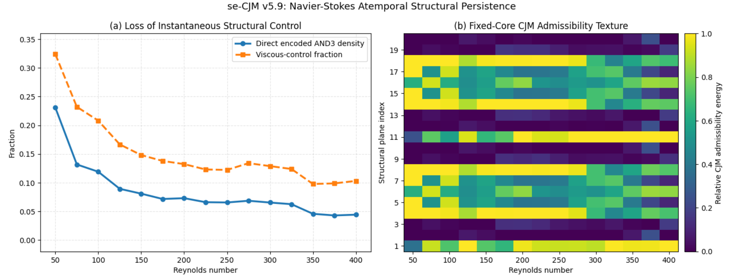
Figure 1: Atemporal structural probe of independently generated three-dimensional Taylor–Green
snapshots. (a) The direct encoded AND3 density and viscous-control fraction decrease substantially
with increasing Reynolds number, indicating loss of instantaneous structural control within the present
encoding. (b) The fixed-core output \(E(Re)=(E_1,\ldots ,E_N)\) is shown as an admissibility texture. Persistent spatial bands
coexist with visible reorganization in the higher-\(Re\) regime. Because each snapshot is independently
median-centered and normalized, color represents within-snapshot organization rather than a common
absolute energy scale. No critical Reynolds number or singularity threshold is inferred.
To examine this possibility numerically, we apply the CJM probe to three-dimensional Taylor–Green flow
[6] on the periodic domain \([0,2\pi ]^3\), with
\begin{equation} \begin {aligned} u_x &= \sin x \cos y \cos z,\\ u_y &= -\cos x \sin y \cos z,\\ u_z &= 0. \end {aligned} \end{equation}
Reference states are generated using a pseudo-spectral incompressible Navier–Stokes solver on a \(20^3\) grid with
\(2/3\)-rule dealiasing [7] and SSP-RK3 integration [8]. Independent cases span \(Re=50,75,\ldots ,400\), with \(\nu =1/Re\), reference time \(t_0=4\), and \(\Delta t=0.02\). The
common reference time permits comparison of structural responses across changing Reynolds-number
conditions. Temporal integration is used only to generate each supplied snapshot \(u_{Re}(x,t_0)\); no subsequent trajectory
information enters the CJM discrimination stage.
Conceptually, each snapshot is treated as a finite global flow configuration,
\begin{equation} u(x,t_0) \longrightarrow \mathcal {G}_{\mathrm {flow}} \longrightarrow (P_\omega ,D_\omega ,x_1,x_2), \end{equation}
where \(\mathcal {G}_{\mathrm {flow}}\) denotes the adopted structural representation of the instantaneous flow. The fields \(P_\omega \) and \(D_\omega \) encode
vortex-stretching and viscous-control information, while \(x_1\) and \(x_2\) provide the finite logic-like interface used by
the CJM core.
Each independently generated representation is then passed through the same fixed CJM
core,
\begin{equation} u_{Re_i}(x,t_0) \longrightarrow \mathcal {G}_{\mathrm {flow}} \longrightarrow (x_1,x_2) \longrightarrow E(Re_i). \end{equation}
No CJM output from another Reynolds-number state is required. The sweep therefore consists of
independent structural discriminations rather than a sequential CJM trajectory. This distinction provides the
operational atemporal component of the present probe: physical states are generated in time, but their CJM
discrimination does not propagate from one flow state to the next.
Figure 3(a) shows a rapid decline in both the viscous-control fraction and encoded AND3 density as \(Re\)
increases. Within the adopted representation, this indicates a systematic reduction of instantaneous structural
control. The two quantities are constructed differently, yet their concurrent decline establishes a common
structural trend across the Reynolds-number sweep.
Figure 3(b) retains information that is lost in a scalar summary. Each column is the independently
discriminated vector
\begin{equation} E(Re_i) = \left ( E_1(Re_i), \ldots , E_N(Re_i) \right ). \end{equation}
Persistent spatial bands remain visible across the scan while their relative intensity and distribution
reorganize at higher \(Re\). Because the response is independently median-centered and normalized within each
snapshot, the relevant comparison is the organization of the texture rather than an absolute energy difference
between columns.
The central observation is therefore the coexistence of two effects: instantaneous structural control
declines, while an organized CJM response does not disappear uniformly. Instead, it persists in a reorganized
form. This persistence is the experimental object considered here. It is not identified with mathematical
regularity itself, nor is any Reynolds number designated as a Changbal threshold or singular
boundary.
The result should therefore be read in relation to the larger atemporal question introduced above. The
experiment does not yet discriminate \(\Phi _{\mathrm {NS}}\) as TRUE or FALSE. It tests whether structural organization relevant
to such a future discrimination can remain observable in a supplied instantaneous state before the subsequent
trajectory is known.
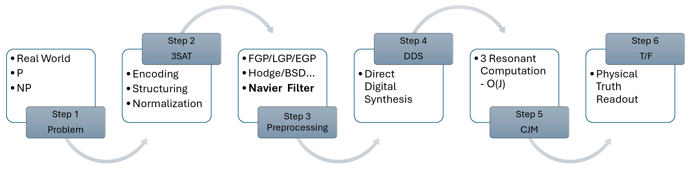
Figure 2: Revised 6-step CJM architecture with the Navier Filter incorporated into Step 3
(Preprocessing). The filter acts as an optional auxiliary gate between Navier–Stokes-inspired 3SAT
structuring and deeper CJM evaluation, and may be bypassed when problem-specific structural
screening is unnecessary. Its operation is defined in Appendix 2 by a six-step conceptual pseudocode:
flow-state signalization, vorticity–strain indicator encoding, 3SAT translation, structural-persistence
screening, admissibility scoring, and final Navier decision. The figure shows where the Navier Filter
may be placed in the pipeline, while the appendix explains how it screens translated flow-state profiles
for structural persistence and admissibility.
4 CJM–Navier: An Optional Structural Filter
The common CJM architecture is organized conceptually as [1]
\begin{equation} \begin {gathered} \mathrm {Problem} \rightarrow \mathrm {3SAT} \\ \rightarrow \mathrm {Preprocessing} \rightarrow \mathrm {DDS} \\ \rightarrow \mathrm {CJM} \rightarrow \mathrm {Readout}. \end {gathered} \end{equation}
Within this architecture, the preprocessing stage provides a modular position for problem-specific
structural representation. Earlier applications used this position for Hodge and BSD filters; here the same
principle is extended to nonlinear flow through a Navier Filter. The filter remains optional and may be
bypassed through the identity operator,
\begin{equation} \mathcal {F}_{\Phi } \in \left \{ \mathcal {F}_{\mathrm {Hodge}}, \mathcal {F}_{\mathrm {BSD}}, \mathcal {F}_{\mathrm {Navier}}, I \right \}, \end{equation}
where \(I\) denotes direct passage to the downstream CJM stages. The Navier Filter therefore
neither defines nor modifies the common CJM core. Its role is to construct a finite Navier-specific
structural interface through which an evolutionary flow state can enter the common discrimination
architecture.
For the present implementation, an instantaneous flow state \(u(x,t_0)\) is treated as a supplied global configuration.
We compute the vorticity and strain tensor [9],
\begin{equation} \omega =\nabla \times u, \qquad S= \frac {1}{2} \left ( \nabla u+\nabla u^{T} \right ), \end{equation}
and construct two structural quantities,
\begin{equation} P_{\omega } = \omega \cdot S\omega , \qquad D_{\omega } = \nu |\nabla \omega |^{2}. \end{equation}
Here \(P_{\omega }\) represents local vortex-stretching production [10], while \(D_{\omega }\) is used as a positive viscous structural
proxy. It is not the exact pointwise diffusive contribution; on a periodic domain,
\begin{equation} \int \omega \cdot \Delta \omega \,dV = - \int |\nabla \omega |^{2}\,dV, \end{equation}
as follows from the standard periodic enstrophy balance [2].
These continuous quantities are mapped into logic-like structural literals,
\begin{equation} x_{1}=1 \quad \Longleftrightarrow \quad P_{\omega }>0, \end{equation}
and
\begin{equation} x_{2}=1 \quad \Longleftrightarrow \quad D_{\omega } \geq \max (P_{\omega },0). \end{equation}
Thus \(x_1\) marks regions of positive vortex stretching, while \(x_2\) marks locations where the viscous proxy is at
least comparable to the positive stretching contribution. In this sense,
\begin{equation} u(x,t_0) \longrightarrow \mathcal {G}_{\mathrm {flow}} \longrightarrow (P_{\omega },D_{\omega }) \longrightarrow (x_1,x_2) \end{equation}
provides the operational structural lift used in the present study. The pair \((x_1,x_2)\) is not itself a proof-theoretic
reduction of the full Navier–Stokes regularity proposition. Rather, it is the finite interface through which flow
organization is exposed to the common CJM discrimination layer.
After this Navier-specific transformation, the downstream CJM core is kept fixed. For the AND3
interaction used here,
\begin{equation} C_i = x_{1,i} \wedge x_{2,i} \wedge x_{1,i-1}, \end{equation}
where \(i-1\) denotes an adjacent structural element within the same snapshot, not a preceding time state. The
distinction is essential: spatial adjacency is encoded inside one supplied configuration, whereas temporal
succession is not used as an input to the CJM core.
The fixed median-centered CJM contrast map then produces
\begin{equation} E(Re) = \left ( E_1,E_2,\ldots ,E_N \right ). \end{equation}
The full vector is retained because its internal organization is central to the present analysis. Scalar
summaries are defined by
\begin{equation} M_J=\operatorname {mean}(E), \qquad D_J=\operatorname {std}(E), \end{equation}
and the periodic median-crossing fragmentation rate
\begin{equation} \begin {aligned} F_J &= \frac {1}{N} \sum _{j=1}^{N} \mathbf {1} \left [ b_j\neq b_{j-1} \right ],\\ b_j &= \mathbf {1} \left [ E_j>\operatorname {median}(E) \right ]. \end {aligned} \end{equation}
These scalar quantities remain secondary diagnostics. The principal object is the organization of the full
admissibility texture and how that organization persists or reorganizes under changes in the supplied flow
state.
The operational CJM–Navier path is therefore summarized as
\begin{equation} \begin {gathered} u_{Re_i}(x,t_0) \rightarrow \mathcal {F}_{\mathrm {Navier}} \rightarrow (x_1,x_2) \\[2pt] \rightarrow \mathrm {CJM} \rightarrow E(Re_i). \end {gathered} \end{equation}
Each Reynolds-number state is evaluated independently, without requiring a preceding or future CJM
state. This snapshot-level construction is not the final discrimination of the global proposition \(\Phi _{\mathrm {NS}}\); it provides a
finite structural pathway toward that stronger objective. The Navier Filter remains an optional
problem-specific lens, while the common CJM core and its atemporal discrimination principle remain
unchanged.
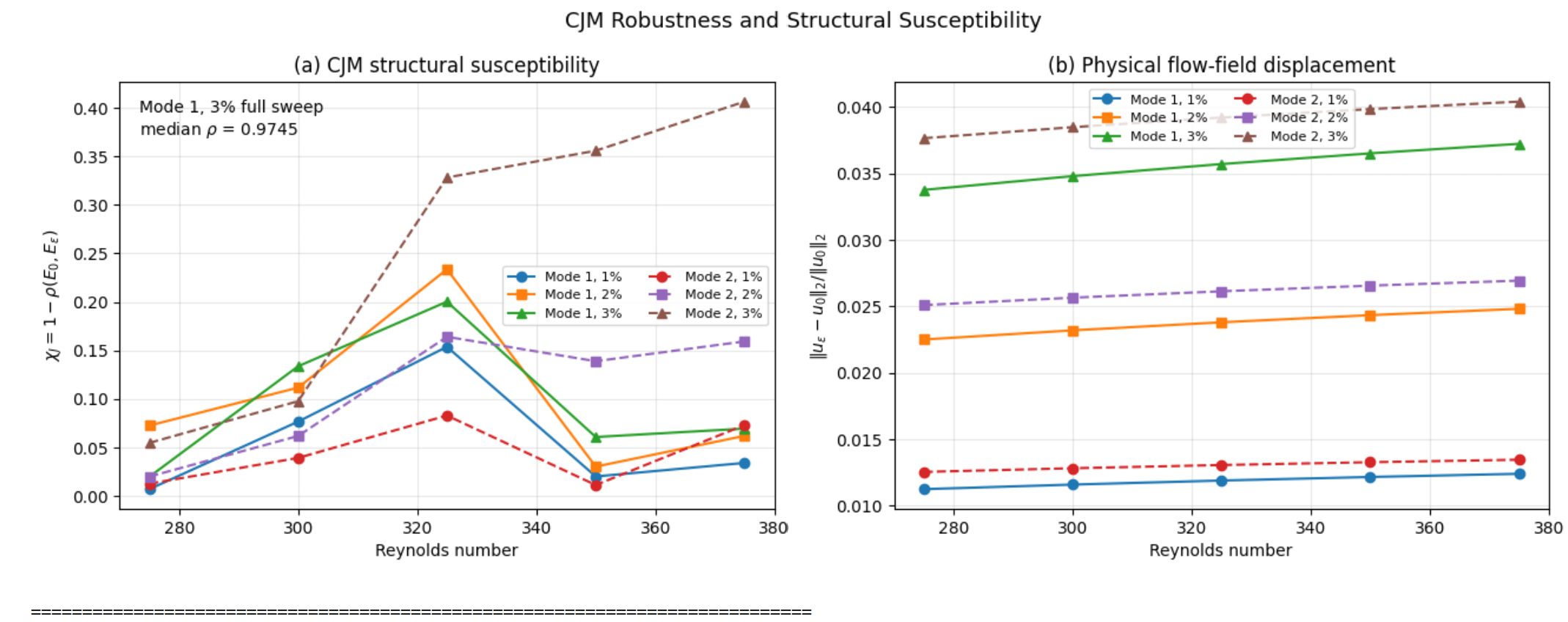
Figure 3: Robustness and structural susceptibility under two independent divergence-free
symmetry-breaking perturbations. (a) Finite CJM structural susceptibility \(\chi _J=1-\rho (E_0,E_{\varepsilon })\) for perturbation
amplitudes of \(1\%\), \(2\%\), and \(3\%\). Mode 1 shows a localized increase near \(Re\approx 325\), while Mode 2 develops a broader
higher-\(Re\) susceptibility, most clearly at \(3\%\). The full-sweep Mode 1 \(3\%\) test retains a median correlation of \(0.9745\). (b)
The corresponding relative physical flow-field displacement changes smoothly with Reynolds number
for both perturbation modes. The contrast indicates nonuniform structural sensitivity of the CJM
representation rather than a corresponding abrupt change in physical flow-field distance. No unique
critical Reynolds number, singularity threshold, or turbulence transition is inferred.
5 Robustness and Structural Susceptibility
To test whether the structure in Figure 3 depends only on exact Taylor–Green symmetry, we introduce small
divergence-free perturbations while keeping the solver, structural encoding, Reynolds-number conditions, and
fixed CJM core unchanged,
\begin{equation} u^{(\varepsilon )} = u_{\mathrm {TG}} + \varepsilon \widehat {\delta u}, \qquad \nabla \cdot \widehat {\delta u}=0. \end{equation}
Two independent symmetry-breaking perturbation modes are examined. A \(3\%\) RMS perturbation using the
first mode across the full Reynolds-number sweep preserves the principal CJM organization, with a median
baseline–perturbed correlation of
\begin{equation} \operatorname {median} \left [ \rho (E_0,E_{\varepsilon }) \right ] = 0.9745. \end{equation}
The high median correlation indicates that the observed admissibility organization is not destroyed
by a small departure from exact Taylor–Green symmetry. At the same time, the response is
not completely rigid: localized reconfiguration remains visible at particular Reynolds-number
conditions.
A focused test is therefore performed with both perturbation modes over \(Re=275\)–\(375\) and amplitudes of \(1\%\)–\(3\%\). We define
the finite structural susceptibility
\begin{equation} \chi _J(Re,\varepsilon ) = 1- \rho \left ( E_0(Re),E_{\varepsilon }(Re) \right ), \end{equation}
so that larger \(\chi _J\) indicates stronger reorganization of the fixed-core CJM texture relative to the unperturbed
baseline.
Figure 3 compares this structural response with the corresponding physical displacement of the flow field.
Panel (a) shows that \(\chi _J\) varies nonuniformly with Reynolds number and depends on both perturbation
mode and amplitude. Mode 1 exhibits a pronounced localized increase near \(Re\approx 325\), whereas Mode 2,
particularly at \(3\%\), develops a broader increase beginning near the same region and continuing toward
higher \(Re\). Panel (b), in contrast, shows that the relative physical flow-field displacement changes
smoothly and nearly monotonically across the same Reynolds-number interval. The contrast is
therefore not simply a consequence of a larger imposed perturbation at one particular Reynolds
number.
Schematically,
\begin{equation} \text {smooth physical change} \not \Longrightarrow \text {smooth CJM response}. \end{equation}
The two perturbation modes do not identify a unique critical Reynolds number. Instead,
they indicate a mode-dependent regime of enhanced structural susceptibility emerging in the
higher-\(Re\) portion of the present sweep. This is consistent with the coexistence of persistence and
selective reorganization: the admissibility texture remains recognizable under small perturbations,
while its internal organization can become substantially more sensitive under particular flow
conditions.
Part of this sensitivity may arise from threshold crossings in the binary definitions of \(x_1\) and \(x_2\). The observed
susceptibility is therefore interpreted as a property of the present finite CJM probe, not as evidence of
a Navier–Stokes singularity, turbulence transition, or mathematically distinguished Reynolds
number.
6 Structural Interpretation and Limitations
Figures 3 and 4 together show two related tendencies. As Reynolds number increases, the selected
viscous-control fraction declines, while the fixed-core CJM organization persists, reorganizes, and becomes
selectively more sensitive to small perturbations. Schematically,
\begin{equation} \begin {gathered} \text {distributed structural control} \\[-1pt] \downarrow \\[-1pt] \text {reduced control} \\[-1pt] \downarrow \\[-1pt] \text {persistent but susceptible organization}. \end {gathered} \end{equation}
This interpretation is structural rather than dynamical. Structural persistence does not imply that the
flow becomes static or that all of its organization is preserved. It refers to the continued detectability of an
organized admissibility texture as the selected instantaneous control measures decrease [10]. The perturbation
tests further show that this organization can remain recognizable while undergoing nonuniform
reconfiguration.
The observed persistence and susceptibility are not identified with singularity, finite-time blow-up,
turbulence, instability, or loss of regularity [5]. In particular, the perturbation experiments do not
establish a unique critical Reynolds number. The present result is instead the coexistence of
declining structural control, persistent organization, and enhanced sensitivity within a finite CJM
representation.
The probe remains limited by its \(20^3\) resolution, finite Reynolds-number interval, fixed reference time \(t_0=4\), small
number of perturbation modes, and direction-dependent spatial encoding. Taylor–Green flow is known to
develop increasingly complex small-scale structure through three-dimensional vortex stretching [11].
Higher resolutions, additional flow states and times, independent perturbations, and equivalent \(x\)-,
\(y\)-, and \(z\)-oriented encodings are therefore required to test numerical, structural, and rotational
robustness.
The binary definitions of \(x_1\) and \(x_2\) also introduce sharp encoding boundaries, so part of the measured
susceptibility may arise from threshold crossings rather than from a distinct physical transition. Likewise, the
independently normalized CJM texture represents within-snapshot organization rather than a common
absolute energy scale.
Finally, the reference snapshots are generated through conventional temporal integration. Atemporality
applies only to the subsequent structural discrimination: the CJM judgment does not require sequential
propagation from preceding to future CJM states. It therefore neither removes physical time from
Navier–Stokes dynamics nor implies hypercomputation. The Navier Filter remains an optional finite
structural interface, and the present probe remains an operational precursor rather than the final
TRUE/FALSE discrimination of \(\Phi _{\mathrm {NS}}\).
7 Conclusion
This paper reconsidered the three-dimensional Navier–Stokes regularity problem as a question of
atemporal structural discrimination. The ultimate CJM–Navier question is whether global smooth
continuation can be discriminated as structurally admissible or inadmissible without requiring
the future trajectory to be sequentially generated as the route to that judgment [4]. Physical
evolution remains temporal, but structural discrimination is conceptually separated from trajectory
generation.
The present study does not yet perform this final TRUE/FALSE discrimination. Instead, it examines a
finite operational precursor. In the three-dimensional Taylor–Green probe [6], increasing Reynolds number is
accompanied by declining instantaneous structural control, while the fixed-core CJM response retains an
organized but reorganized admissibility texture. The principal observation is thus the coexistence of reduced
control with persistent structural organization.
The perturbation experiments extend this result. A \(3\%\) Mode 1 symmetry-breaking perturbation retains a
median baseline–perturbed correlation of \(0.9745\), indicating substantial robustness. At the same time, Mode 1 shows
a localized increase in susceptibility near \(Re\approx 325\), whereas Mode 2 develops a broader higher-\(Re\) response.
The sensitivity is therefore mode-dependent and does not identify a unique critical Reynolds
number.
Across the same interval, the physical velocity-field displacement changes smoothly, while the CJM
susceptibility varies nonuniformly. Within the present representation,
\begin{equation} \begin {gathered} \text {smooth physical change} \\ \not \Longrightarrow \; \text {smooth structural response}. \end {gathered} \end{equation}
The result therefore supports a combined picture of structural persistence and structural susceptibility,
rather than evidence for a new physical transition [11]. CJM–Navier is accordingly interpreted as an optional
problem-specific structural interface within the common CJM architecture [1], not as a replacement for the
Navier–Stokes equations or a direct regularity criterion.
Important limitations remain. The present calculations use a \(20^3\) grid, a finite Reynolds-number
interval, a fixed sampling time, two perturbation modes, and a direction-dependent binary encoding.
Threshold crossings in \(x_1\) and \(x_2\) may also contribute to the measured susceptibility. No claim of
global smoothness, finite-time singularity, or critical Reynolds number is therefore made [12].
Higher resolution, alternative flow states, spatial encodings, and broader perturbation tests remain
necessary.
The deeper question remains whether Navier–Stokes regularity can ultimately be characterized not only
through the temporal survival of a trajectory, but through the structural admissibility of that continuation
before the trajectory is known. The flow evolves in time; CJM asks whether the truth of its global
continuation must also be reached through time.
Open Question.
Does a problem \(\Phi \) admit a solution if and only if it is structurally admissible under atemporal
resonance?
References
-
[1]
- Yoon, K. (2025). \(P \equiv NP^{J}\): On the End of Time.
-
[2]
- Constantin, P., & Foias, C. (1988). Navier–Stokes Equations. Chicago Lectures in Mathematics.
University of Chicago Press.
-
[3]
- Fefferman, C. L. (2000). Existence and Smoothness of the Navier–Stokes Equation. Clay
Mathematics Institute.
-
[4]
- Kato, T. (1984). Strong \(L^p\)-Solutions of the Navier–Stokes Equation in \(\mathbb {R}^m\), with Applications to Weak
Solutions. Mathematische Zeitschrift, 187, 471–480.
-
[5]
- Serrin, J. (1962). On the Interior Regularity of Weak Solutions of the Navier–Stokes Equations.
Archive for Rational Mechanics and Analysis, 9, 187–195.
-
[6]
- Taylor, G. I., & Green, A. E. (1937). Mechanism of the Production of Small Eddies from Large
Ones. Proceedings of the Royal Society of London. Series A, 158(895), 499–521.
-
[7]
- Orszag, S. A. (1971). On the Elimination of Aliasing in Finite-Difference Schemes by Filtering
High-Wavenumber Components. Journal of the Atmospheric Sciences, 28(6), 1074.
-
[8]
- Gottlieb, S., & Shu, C.-W. (1998). Total Variation Diminishing Runge–Kutta Schemes.
Mathematics of Computation, 67(221), 73–85.
-
[9]
- Majda, A. J., & Bertozzi, A. L. (2002). Vorticity and Incompressible Flow. Cambridge Texts in
Applied Mathematics, Vol. 27. Cambridge University Press.
-
[10]
- Doering, C. R., & Gibbon, J. D. (1995). Applied Analysis of the Navier–Stokes Equations.
Cambridge Texts in Applied Mathematics, Vol. 12. Cambridge University Press.
-
[11]
- Brachet, M. E., Meiron, D. I., Orszag, S. A., Nickel, B. G., Morf, R. H., & Frisch, U. (1983).
Small-Scale Structure of the Taylor–Green Vortex. Journal of Fluid Mechanics, 130, 411–452.
-
[12]
- Caffarelli, L., Kohn, R., & Nirenberg, L. (1982). Partial Regularity of Suitable Weak Solutions of
the Navier–Stokes Equations. Communications on Pure and Applied Mathematics, 35(6), 771–831.
def make_spectral_grid(N):

    k = np.fft.fftfreq(N, d=1.0 / N)

    KX, KY, KZ = np.meshgrid(
        k, k, k,
        indexing="ij"
    )

    K2 = (
        KX**2
        +
        KY**2
        +
        KZ**2
    )

    K2_SAFE = K2.copy()
    K2_SAFE[0, 0, 0] = 1.0

    K_MAG = np.sqrt(K2)

    K_CUT = N // 3

# Full code available at the links below (Colab, GitHub, project website).
Appendix 2: Navier Filter
Pseudocode
PROCEDURE step1_input_navier_filter(input_instance):

    # Interpret the input according to its current physical or logical form
    IF input_instance is FlowSnapshot u(x,t0):
        U <- ExtractInstantaneousFlowState(u(x,t0))
        Sigma_N <- BuildNavierStructural
        Representation(U)

    ELSE IF input_instance is NavierIndicatorProfile Theta_N:
        Sigma_N <- LiftToNavierStructural
        Representation(Theta_N)

    ELSE IF input_instance is Navier3SATFormula F:
        Sigma_N <- LiftToNavierStructural
        Representation(F)

    ELSE IF input_instance is SATReducedInstance F:
        Sigma_N <- LiftToNavierStructural
        Representation(F)

# Full code available at the links below (Colab, GitHub, project website).
def make_spectral_grid(N):
    k = np.fft.fftfreq(N, d=1.0 / N)
    KX, KY, KZ = np.meshgrid(k, k, k, indexing="ij")

    K2 = KX**2 + KY**2 + KZ**2
    K2_SAFE = K2.copy()
    K2_SAFE[0, 0, 0] = 1.0

    K_CUT = N // 3
    DEALIAS = (
        (np.abs(KX) <= K_CUT)
        & (np.abs(KY) <= K_CUT)
        & (np.abs(KZ) <= K_CUT)
    )

    return KX, KY, KZ, K2, K2_SAFE, DEALIAS


def project_divergence_free(u_hat, KX, KY, KZ, K2_SAFE):
    k_dot_u = KX * u_hat[0] + KY * u_hat[1] + KZ * u_hat[2]

    out = u_hat.copy()
    out[0] -= KX * k_dot_u / K2_SAFE
    out[1] -= KY * k_dot_u / K2_SAFE
    out[2] -= KZ * k_dot_u / K2_SAFE

    out[:, 0, 0, 0] = 0.0
    return out


# Full code available at the links below (Colab, GitHub, project website).